Tobit models handle left-censored data by combining cumulative probability mass with continuous normal densities

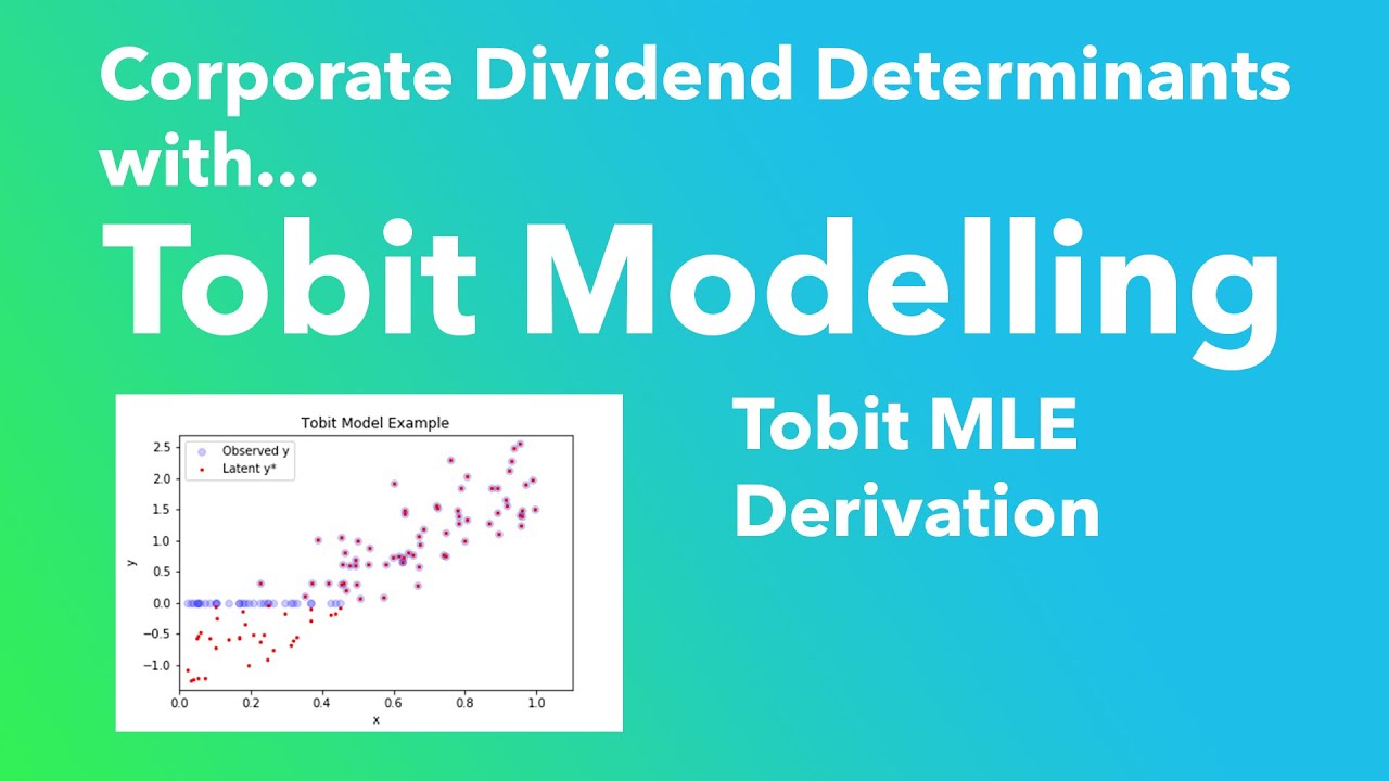
I cover the mathematical derivation of the Maximum Likelihood Estimation (MLE) log-likelihood function for the Tobit model under left-censoring.

The idea

Standard Ordinary Least Squares (OLS) regression fails when dependent variables are censored or bounded at a threshold (e.g., zero wage or minimum price floors), producing biased parameter estimates. The Tobit model addresses this by introducing an unobserved continuous latent variable $y_i^*$ generated by a linear regression process. When the latent variable falls below a threshold $C$, the observed response $y_i$ is clamped at $C$; otherwise, $y_i$ equals $y_i^*$.

To estimate model parameters via Maximum Likelihood Estimation, the density function must be partitioned into two components: a discrete probability mass for observations at the censoring threshold and a continuous normal probability density for uncensored observations. By combining these terms into a single joint likelihood using indicator dummy variables, we formulate a differentiable log-likelihood objective.

The mechanism

This defines the Tobit framework where $y_i^*$ is a latent variable and observed $y_i$ is left-censored at threshold $C$.

This calculates the cumulative distribution function (CDF) mass for observations that fall at or below the censoring limit $C$.

This calculates the standard normal probability density function (PDF) for uncensored observations above threshold $C$.

This defines the average log-likelihood function optimized to find MLE estimates for parameters $\beta$ and $\sigma$, where $d_i = \mathbb{I}(y_i = C)$.

Worth knowing

• Standard linear regression yields biased parameter estimates on censored data because it ignores the probability accumulation at threshold $C$.
• The censoring threshold $C$ is general and can represent zero, minimum wages, or price floors rather than strictly zero.
• The likelihood function is a hybrid mixture: a discrete probability mass function for $y_i = C$ and a continuous probability density for $y_i > C$.
• Using an indicator variable $d_i \in \{0, 1\}$ allows combining both piece-wise density conditions into a single continuous product before taking logarithms.

Mathematical derivation steps

1. Define latent model: Express $y_i^* = x_i^T \beta + \epsilon_i$ with normal error $\epsilon_i \sim \mathcal{N}(0, \sigma^2)$.
2. Derive linear regression PDF: Express CDF $F(y_i) = P(\epsilon_i \le y_i - x_i^T \beta) = \Phi\left(\frac{y_i - x_i^T \beta}{\sigma}\right)$ and differentiate with respect to $y_i$ to obtain $f(y_i) = \frac{1}{\sigma}\phi\left(\frac{y_i - x_i^T \beta}{\sigma}\right)$.
3. Partition density function:
   • For $y_i < C$: density is $0$.
   • For $y_i = C$: mass is $P(y_i^* \le C) = \Phi\left(\frac{C - x_i^T \beta}{\sigma}\right)$.
   • For $y_i > C$: density is $\frac{1}{\sigma}\phi\left(\frac{y_i - x_i^T \beta}{\sigma}\right)$.
4. Construct individual likelihood: Define indicator $d_i = 1$ if $y_i = C$ and $d_i = 0$ if $y_i > C$. Form $L_i = \left[\Phi\left(\frac{C - x_i^T \beta}{\sigma}\right)\right]^{d_i} \left[\frac{1}{\sigma}\phi\left(\frac{y_i - x_i^T \beta}{\sigma}\right)\right]^{1 - d_i}$.
5. Form log-likelihood: Apply logarithm rules to transform products into sums and average over $N$ observations.

Use it when / don't use it when

Use it when

• Dependent variables in your dataset are strictly clustered or censored at a specific lower bound (e.g., $0$).
• You want unbiased estimates of linear model coefficients when working with corner-solution dependent variables like wages or dividend payments.

Don't use it when

• The dependent variable is continuous and unrestricted across the real line.
• Zero or boundary values are generated by a distinct qualitative selection process requiring a hurdle or selection model.

Further reading

• Estimation of Relationships for Limited Dependent Variables (Tobin, 1958)
• Econometric Analysis (Greene)
• Microeconometrics: Methods and Applications (Cameron & Trivedi)