The Mathematics of Hidden Markov Models

Mathematics of Hidden Markov Models: filtering, smoothing, and inference via Expectation-Maximization.

Model Definition

A Hidden Markov Model (HMM) consists of a sequence of hidden states z1:Tz_{1:T} with zt{1,,K}z_t \in \{1,\dots,K\} evolving over time, each generating an observation xtx_t.

p(z1:T,x1:T)=p(z1)t=2Tp(ztzt1)t=1Tp(xtzt)(1)p(z_{1:T}, x_{1:T}) = p(z_{1}) \prod_{t=2}^{T} p(z_{t} \mid z_{t-1}) \prod_{t=1}^{T} p(x_{t} \mid z_{t}) \tag{1}

The factorization encodes two key conditional independence assumptions: (1) the evolution of latent states is 1-Markov, and (2) each observation depends only on the contemporaneous latent state.
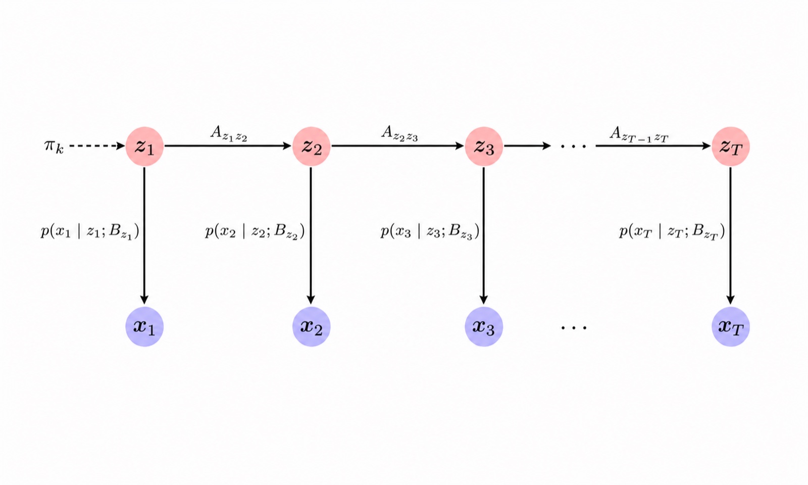
Graphical structure of a Hidden Markov Model

Figure 1: Graphical structure of a Hidden Markov Model. Latent states z1:Tz_{1:T} form a Markov chain, and each observation xtx_t depends only on ztz_t.

Inference

Since only x1:Tx_{1:T} is observed, there are two major inference tasks: (1) filtering p(zt=kx1:t)p(z_t=k \mid x_{1:t}) and (2) smoothing p(zt=kx1:T)p(z_{t}=k \mid x_{1:T}). With smoothing, observations beyond state ztz_t are used to compute the posterior. From these results, other tasks like future latent states or observations become straightforward. We will first look at filtering.

Filtering: Inferring Current Latent State

Filtering is the task of computing the posterior p(zt=kx1:t)p(z_t=k \mid x_{1:t}) over latent states given observations up to time tt. Writing

p(zt=kx1:t)=p(x1:t,zt=k)p(x1:t)(2)p(z_{t}=k \mid x_{1:t}) = \frac{p(x_{1:t}, z_{t}=k)}{p(x_{1:t})} \tag{2}

it suffices to track the numerator p(x1:t,zt=k)p(x_{1:t}, z_{t}=k). Using the conditional independence implied by (1), xt(zt1,x1:t1)ztx_{t} \perp (z_{t-1}, x_{1:t-1}) \mid z_{t} and ztx1:t1zt1z_{t} \perp x_{1:t-1} \mid z_{t-1}, we have

p(x1:t,zt=k)=j=1Kp(zt=k,zt1=j,x1:t)=j=1Kp(xtzt=k)p(zt=kzt1=j)p(zt1=j,x1:t1)=p(xtzt=k)j=1Kp(zt=kzt1=j)p(zt1=j,x1:t1)\begin{align*} p(x_{1:t}, z_{t}=k) &= \sum_{j=1}^{K} p(z_{t}=k, z_{t-1}=j, x_{1:t}) \\ &= \sum_{j=1}^{K} p(x_{t} \mid z_{t}=k)\, p(z_{t}=k \mid z_{t-1}=j)\, p(z_{t-1}=j, x_{1:t-1}) \\ &= p(x_{t} \mid z_{t}=k) \sum_{j=1}^{K} p(z_{t}=k \mid z_{t-1}=j)\, p(z_{t-1}=j, x_{1:t-1}) \end{align*}

Definition (Forward variable). Define αt(k)p(x1:t,zt=k)\alpha_t(k) \equiv p(x_{1:t}, z_t=k) for t1t \geq 1.

Proposition (Forward recursion). The forward variables satisfy, for t2t \geq 2:

αt(k)=p(xtzt=k)j=1Kp(zt=kzt1=j)αt1(j)\alpha_t(k) = p(x_t \mid z_t = k) \sum_{j=1}^{K} p(z_t = k \mid z_{t-1} = j)\, \alpha_{t-1}(j)

for t=1t = 1:

α1(k)=p(x1z1=k)p(z1=k)\alpha_1(k) = p(x_1 \mid z_1 = k)\, p(z_1 = k)

The marginal likelihood (probability of the data) p(x1:t)p(x_{1:t}) can be recovered by summing over the latent states α\alpha:

p(x1:t)=i=1Kp(x1:t,zt=i)=i=1Kαt(i)(3)p(x_{1:t}) = \sum_{i=1}^{K} p(x_{1:t}, z_{t}=i) = \sum_{i=1}^{K} \alpha_{t}(i) \tag{3}

Which gives us

p(zt=kx1:t)=p(xtzt=k)j=1Kp(zt=kzt1=j)αt1(j)i=1Kαt(i)(4)p(z_{t}=k \mid x_{1:t}) = \frac{p(x_{t} \mid z_{t}=k) \displaystyle\sum_{j=1}^{K} p(z_{t}=k \mid z_{t-1}=j)\, \alpha_{t-1}(j)}{\displaystyle\sum_{i=1}^{K} \alpha_{t}(i)} \tag{4}

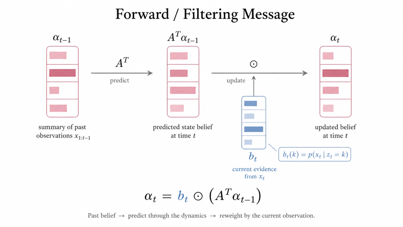
Forward filtering message

Figure 2: Forward filtering message. Filtering alternates between prediction through the transition model and correction by the current observation.

Smoothing: Inferring an Intermediate Latent State

In the context of HMMs, smoothing refers to finding p(ztx1:T)p(z_{t} \mid x_{1:T}), making use of the full observation sequence to infer an intermediate latent state. Intuitively, even observations beyond ztz_t can still carry information about the state of ztz_t through the Markov chain. Starting with the object of interest

p(zt=ix1:T)=p(x1:T,zt=i)p(x1:T)(5)p(z_{t} = i \mid x_{1:T}) = \frac{p(x_{1:T}, z_{t}=i)}{p(x_{1:T})} \tag{5}

Focusing on the numerator:

p(x1:T,zt=i)=p(x1:t,zt=i,xt+1:T)=p(x1:t,zt=i)p(xt+1:Tzt=i)\begin{align*} p(x_{1:T}, z_{t}=i) &= p(x_{1:t}, z_{t}=i, x_{t+1:T}) \\ &= p(x_{1:t}, z_{t}=i)\, p(x_{t+1:T} \mid z_{t}=i) \end{align*}

which is using the conditional independence due to the HMM graph, x1:txt+1:Tztx_{1:t} \perp x_{t+1:T} \mid z_{t}:

=αt(i)p(xt+1:Tzt=i)= \alpha_{t}(i)\, p(x_{t+1:T} \mid z_{t}=i)

Definition (Backward variable). Define βt(i)p(xt+1:Tzt=i)\beta_t(i) \equiv p(x_{t+1:T} \mid z_t = i).

Proposition (Backward recursion). For 1tT11 \leq t \leq T-1:

βt(i)=j=1Kp(xt+1zt+1=j)Aijβt+1(j)\beta_t(i) = \sum_{j=1}^{K} p(x_{t+1} \mid z_{t+1}=j)\, A_{ij}\, \beta_{t+1}(j)

with terminal condition βT(i)=1\beta_T(i) = 1.

Proof.

βt(i)=p(xt+1:Tzt=i)=j=1Kp(xt+1:T,zt+1=jzt=i)=j=1Kp(xt+1,xt+2:T,zt+1=jzt=i)=j=1Kp(xt+1,xt+2:Tzt+1=j,zt=i)p(zt+1=jzt=i)\begin{align*} \beta_t(i) &= p(x_{t+1:T} \mid z_{t}=i) = \sum_{j=1}^{K} p(x_{t+1:T}, z_{t+1}=j \mid z_{t}=i) \\ &= \sum_{j=1}^{K} p(x_{t+1}, x_{t+2:T}, z_{t+1}=j \mid z_{t}=i) \\ &= \sum_{j=1}^{K} p(x_{t+1}, x_{t+2:T} \mid z_{t+1}=j, z_{t}=i)\, p(z_{t+1}=j \mid z_{t}=i) \end{align*}

and now because xt+2:T(xt+1,zt)zt+1x_{t+2:T} \perp (x_{t+1}, z_{t}) \mid z_{t+1} and xt+1ztzt+1x_{t+1} \perp z_t \mid z_{t+1}:

=j=1Kp(xt+1zt+1=j)p(xt+2:Tzt+1=j)βt+1(j)p(zt+1=jzt=i)Aij=j=1Kp(xt+1zt+1=j)Aijβt+1(j)\begin{align*} &= \sum_{j=1}^{K} p(x_{t+1} \mid z_{t+1}=j)\, \underbrace{p(x_{t+2:T} \mid z_{t+1}=j)}_{\beta_{t+1}(j)}\, \underbrace{p(z_{t+1}=j \mid z_{t}=i)}_{A_{ij}} \\ &= \sum_{j=1}^{K} p(x_{t+1} \mid z_{t+1}=j)\, A_{ij}\, \beta_{t+1}(j) \end{align*}

and for t=Tt=T, for convenience we define βT(j)=1\beta_{T}(j) = 1 for j{1,,K}j \in \{1, \ldots, K\}. \square

Definition (Smoother). Define γt(i)p(zt=ix1:T)\gamma_{t}(i) \equiv p(z_{t}=i \mid x_{1:T}).

Proposition (Smoothing distribution). Putting together (5), for any tt,

γt(i)=p(zt=ix1:T)=αt(i)βt(i)j=1Kαt(j)βt(j)\gamma_t(i) = p(z_t=i \mid x_{1:T}) = \frac{\alpha_t(i)\,\beta_t(i)}{\sum_{j=1}^{K} \alpha_t(j)\,\beta_t(j)}

Parameter Fitting

The model parameters consist of the initial state distribution, the transition distribution between latent states, and the emission distribution associated with each latent state.

That is, the model parameters are:

πk=p(z1=k),Ajk=p(zt=kzt1=j),Bk=emission parameters for state k\pi_k = p(z_1 = k), \qquad A_{jk} = p(z_t = k \mid z_{t-1} = j), \qquad B_k = \text{emission parameters for state } k

Following the method of maximum likelihood estimation, we'd like to maximize the probability of the data given the parameters.

θ^=argmaxθΘ logp(Xθ)=argmaxθΘ log(n=1Np(xnθ))=argmaxθΘ log(n=1Nznp(xn,znθ))=argmaxθΘn=1Nlogznp(xn,znθ)\begin{align*} \hat{\boldsymbol{\theta}} &= \operatorname*{argmax}_{\theta \in \Theta}\ \log p(\mathbf{X} \mid \boldsymbol{\theta}) \\ &= \operatorname*{argmax}_{\theta \in \Theta}\ \log \left( \prod_{n=1}^{N} p(\mathbf{x}_{n} \mid \boldsymbol{\theta}) \right) \\ &= \operatorname*{argmax}_{\theta \in \Theta}\ \log \left( \prod_{n=1}^{N} \sum_{\mathbf{z}_n} p(\mathbf{x}_{n}, \mathbf{z}_{n} \mid \boldsymbol{\theta}) \right) \\ &= \operatorname*{argmax}_{\theta \in \Theta} \sum_{n=1}^{N} \log \sum_{\mathbf{z}_n} p(\mathbf{x}_{n}, \mathbf{z}_{n} \mid \boldsymbol{\theta}) \end{align*}

The sum over latent sequences appears inside the logarithm, which couples the parameters across all possible zn\mathbf{z}_n. This prevents the objective from decomposing into separable terms, and hence no closed-form maximizer exists.

Expectation-Maximization - E-step

Under EM we want to maximize the expected complete-data log-likelihood under the current posterior:

Q(θ,θold)=Ep(z1:Tx1:T,θold)[logp(x1:T,z1:Tθ)]=Ep(z1:Tx1:T,θold)[k=1KI(z1=k)logπk+t=2Tj=1Kk=1KI(zt1=j,zt=k)logAjk+t=1Tk=1KI(zt=k)logp(xtzt=k;Bk)]\begin{align*} Q(\theta, \theta^{\text{old}}) &= \mathbb{E}_{p(z_{1:T} \mid x_{1:T}, \theta^{\text{old}})} \left[ \log p(x_{1:T}, z_{1:T} \mid \theta) \right] \\ &= \mathbb{E}_{p(z_{1:T} \mid x_{1:T}, \theta^{\text{old}})} \Biggl[ \sum_{k=1}^{K} \mathbb{I}(z_{1}=k) \log \pi_{k} \\ &\qquad\qquad + \sum_{t=2}^{T} \sum_{j=1}^{K} \sum_{k=1}^{K} \mathbb{I}(z_{t-1}=j, z_{t}=k) \log A_{jk} \\ &\qquad\qquad + \sum_{t=1}^{T} \sum_{k=1}^{K} \mathbb{I}(z_{t}=k) \log p(x_{t} \mid z_{t}=k; B_{k}) \Biggr] \end{align*}

Moving expectations inside:

=k=1Kp(z1=kx1:T)logπk+t=2Tj=1Kk=1Kp(zt1=j,zt=kx1:T)logAjk+t=1Tk=1Kp(zt=kx1:T)logp(xtzt=k;Bk)=k=1Kγ1(k)logπk+t=2Tj=1Kk=1Kξt(j,k)p(zt1=j,zt=kx1:T)logAjk+t=1Tk=1Kγt(k)logp(xtzt=k;Bk)\begin{align*} &= \sum_{k=1}^{K} p(z_{1}=k \mid x_{1:T}) \log \pi_{k} \\ &\qquad + \sum_{t=2}^{T} \sum_{j=1}^{K} \sum_{k=1}^{K} p(z_{t-1}=j, z_{t}=k \mid x_{1:T}) \log A_{jk} \\ &\qquad + \sum_{t=1}^{T} \sum_{k=1}^{K} p(z_{t}=k \mid x_{1:T}) \log p(x_{t} \mid z_{t}=k; B_{k}) \\[6pt] &= \sum_{k=1}^{K} \gamma_{1}(k) \log \pi_{k} \\ &\qquad + \sum_{t=2}^{T} \sum_{j=1}^{K} \sum_{k=1}^{K} \underbrace{\xi_{t}(j,k)}_{p(z_{t-1}=j,\, z_t=k \mid x_{1:T})} \log A_{jk} \\ &\qquad + \sum_{t=1}^{T} \sum_{k=1}^{K} \gamma_{t}(k) \log p(x_{t} \mid z_{t}=k; B_{k}) \end{align*}

Definition (Pairwise Smoother). Define ξt(j,k)p(zt1=j,zt=kx1:T)\xi_{t}(j,k) \equiv p(z_{t-1}=j,\, z_t=k \mid x_{1:T}).

Writing ξt(j,k)\xi_{t}(j,k) in terms of objects we already have:

ξt(j,k)=p(zt1=j,zt=kx1:T)=p(zt1=j,zt=k,x1:T)p(x1:T)=p(zt1=j,zt=k,x1:t1,xt,xt+1:T)p(x1:T)=p(x1:t1,zt1=j)p(zt=kzt1=j)p(xtzt=k)p(xt+1:Tzt=k)p(x1:T)=αt1(j)Ajkp(xtzt=k)βt(k)i=1Kαt(i)βt(i)\begin{align*} \xi_{t}(j,k) &= p(z_{t-1}=j, z_{t}=k \mid x_{1:T}) \\ &= \frac{p(z_{t-1}=j, z_{t}=k, x_{1:T})}{p(x_{1:T})} \\ &= \frac{p(z_{t-1}=j, z_{t}=k, x_{1:t-1}, x_{t}, x_{t+1:T})}{p(x_{1:T})} \\ &= \frac{p(x_{1:t-1}, z_{t-1}=j)\, p(z_{t}=k \mid z_{t-1}=j)\, p(x_{t} \mid z_{t}=k)\, p(x_{t+1:T} \mid z_{t}=k)}{p(x_{1:T})} \\ &= \frac{\alpha_{t-1}(j)\, A_{jk}\, p(x_{t} \mid z_{t}=k)\, \beta_{t}(k)}{\sum_{i=1}^{K} \alpha_{t}(i)\, \beta_{t}(i)} \end{align*}

To summarize:

Q(θ,θold)=kγ1(k)logπkQπ+t=2Tj,kξt(j,k)logAjkQA+t=1Tkγt(k)logp(xtzt=k;Bk)QBQ(\theta, \theta^{\text{old}}) = \underbrace{\sum_{k} \gamma_1(k) \log \pi_k}_{Q_{\pi}} + \underbrace{\sum_{t=2}^{T} \sum_{j,k} \xi_t(j,k) \log A_{jk}}_{Q_{A}} + \underbrace{\sum_{t=1}^{T} \sum_{k} \gamma_t(k) \log p(x_t \mid z_t=k; B_k)}_{Q_{B}}

We have now computed the expectation of the log-likelihood under the posterior of the latent variables.

Expectation Maximization - M-step

Now, we need to update the parameters of our model θ=(π,A,B)\theta = (\pi, A, B). Since QQ is the sum of three terms of distinct parameters, we can maximize each term independently. Starting with maximizing the first term QπQ_{\pi}:

Initial distribution.

Qπ=kγ1(k)logπksubject to kπk=1Q_{\pi} = \sum_{k} \gamma_1(k) \log \pi_k \quad \text{subject to } \sum_{k} \pi_{k} = 1

Setting up the Lagrangian:

L(π,λ)=k=1Kγ1(k)logπk+λ(k=1Kπk1)Lπk=γ1(k)πk+λ=0πk=γ1(k)λ\begin{align*} \mathcal{L}(\pi, \lambda) &= \sum_{k=1}^{K} \gamma_{1}(k) \log \pi_{k} + \lambda \left( \sum_{k=1}^{K} \pi_{k} - 1 \right) \\ \frac{\partial \mathcal{L}}{\partial \pi_{k}} &= \frac{\gamma_{1}(k)}{\pi_{k}} + \lambda = 0 \\ \pi_{k} &= \frac{-\gamma_{1}(k)}{\lambda} \end{align*}

Now using the constraint:

k=1Kπk=1    kγ1(k)λ=1\sum_{k=1}^{K} \pi_{k} = 1 \implies \sum_{k} \frac{-\gamma_{1}(k)}{\lambda} = 1

and because γ1(k)p(z1=kx1:T)\gamma_{1}(k) \equiv p(z_{1}=k \mid x_{1:T}) the sum across all latent states kp(z1=kx1:T)=1\sum_{k} p(z_{1}=k \mid x_{1:T}) = 1 and hence

λ=1    πknew=γ1(k)\lambda = -1 \implies \boxed{\pi_{k}^{\text{new}} = \gamma_{1}(k)}

Now we take a brief detour to prove a classic result which can be reused.

Lemma. The solution to maxpkwklogpk\max_p \sum_k w_k \log p_k subject to kpk=1\sum_k p_k = 1, pk0p_k \geq 0, is

pk=wkjwjp_k = \frac{w_k}{\sum_j w_j}

Proof. From the Lagrangian L(p,λ)=kwklogpk+λ(kpk1)\mathcal{L}(p, \lambda) = \sum_{k} w_{k} \log p_{k} + \lambda (\sum_{k} p_{k} - 1), take the derivative w.r.t. pkp_{k}: Lpk=wkpk+λ=0\frac{\partial \mathcal{L}}{\partial p_{k}} = \frac{w_{k}}{p_{k}} + \lambda = 0. Solving: wkpk=λ    pk=wkλ    λ=kwk\frac{w_{k}}{p_{k}} = -\lambda \implies p_{k} = \frac{w_{k}}{-\lambda} \implies -\lambda = \sum_{k} w_{k}. The constraint kpk=1\sum_k p_k = 1 then forces pk=wkjwjp_{k} = \frac{w_{k}}{\sum_{j} w_{j}}. \square

Transition matrix. The result applies to QAQ_{A}:

QA=t=2Tj,kξt(j,k)logAjk=jkt=2Tξt(j,k)logAjk\begin{align*} Q_{A} &= \sum_{t=2}^{T} \sum_{j,k} \xi_t(j,k) \log A_{jk} \\ &= \sum_{j} \sum_{k} \sum_{t=2}^{T} \xi_t(j,k) \log A_{jk} \end{align*}

Considering a particular jj we'd like to maximize

kt=2Tξt(j,k)logAjks.t. k=1KAjk=1\sum_{k} \sum_{t=2}^{T} \xi_t(j,k) \log A_{jk} \quad \text{s.t. } \sum_{k=1}^{K} A_{jk} = 1

Making use of the Lemma, we see this is maximized by

Ajk=t=2Tξt(j,k)i=1Kt=2Tξt(j,i)A_{jk} = \frac{\sum_{t=2}^{T} \xi_{t}(j,k)}{\sum_{i=1}^{K}\sum_{t=2}^{T} \xi_{t}(j,i)}

and because

i=1Kt=2Tξt(j,i)=t=2Ti=1Kξt(j,i)=t=2Ti=1Kp(zt=i,zt1=jx1:T)=t=2Tp(zt1=jx1:T)=t=2Tγt1(j)\begin{align*} \sum_{i=1}^{K}\sum_{t=2}^{T} \xi_{t}(j,i) &= \sum_{t=2}^{T} \sum_{i=1}^{K} \xi_{t}(j,i) \\ &= \sum_{t=2}^{T} \sum_{i=1}^{K} p(z_{t}=i, z_{t-1}=j \mid x_{1:T}) \\ &= \sum_{t=2}^{T} p(z_{t-1}=j \mid x_{1:T}) \\ &= \sum_{t=2}^{T} \gamma_{t-1}(j) \end{align*}

Therefore, substituting this result into the denominator:

Ajknew=t=2Tξt(j,k)t=2Tγt1(j)(6)\boxed{A_{jk}^{\text{new}} = \frac{\sum_{t=2}^{T} \xi_{t}(j,k)}{\sum_{t=2}^{T} \gamma_{t-1}(j)}} \tag{6}

Remark. The updated transition parameters become the normalized estimated/"soft" (from the E-step) counts of transitions from jkj \to k.

The final term to deal with is the emission parameters. The optimization depends on whether we choose emission to be categorical, Gaussian, or some other distribution. For a categorical distribution, we can follow a similar approach using the general result as we did with QAQ_{A} and QπQ_{\pi}.

Let us also show the derivation for Gaussian emissions.

Emission parameters (Gaussian).

QB=t=1Tkγt(k)logp(xtzt=k;Bk)=t=1Tkγt(k)[(xtμk)22σk2log(σk2π)]=kt=1Tγt(k)[(xtμk)22σk2log(σk2π)]\begin{align*} Q_{B} &= \sum_{t=1}^{T} \sum_{k} \gamma_{t}(k) \log p(x_{t} \mid z_{t}=k; B_{k}) \\ &= \sum_{t=1}^{T} \sum_{k} \gamma_{t}(k) \left[ -\frac{(x_t - \mu_k)^2}{2\sigma_k^2} - \log\left(\sigma_k \sqrt{2\pi}\right) \right] \\ &= \sum_{k} \sum_{t=1}^{T} \gamma_{t}(k) \left[ -\frac{(x_t - \mu_k)^2}{2\sigma_k^2} - \log\left(\sigma_k \sqrt{2\pi}\right) \right] \end{align*}

Let's start by finding μk\mu_{k}:

QBμk=t=1Tγt(k)[xtμkσk2]=0    t=1Tγt(k)(xtμk)=0    μknew=t=1Tγt(k)xtt=1Tγt(k)\begin{align*} \frac{\partial Q_{B}}{\partial \mu_{k}} &= \sum_{t=1}^{T} \gamma_{t}(k) \left[ \frac{x_{t} - \mu_{k}}{\sigma_{k}^{2}} \right] = 0 \\ &\implies \sum_{t=1}^{T} \gamma_{t}(k) \left( x_{t} - \mu_{k}\right) = 0 \\ &\implies \boxed{\mu_{k}^{\text{new}} = \frac{\sum_{t=1}^{T} \gamma_{t}(k) x_{t}}{\sum_{t=1}^{T} \gamma_{t}(k)}} \tag{7} \end{align*}

Now, solving for the variance term:

QBσk=t=1Tγt(k)[(xtμk)2σk31σk]=0    σk2t=1Tγt(k)=t=1Tγt(k)(xtμk)2    (σk2)new=t=1Tγt(k)(xtμknew)2t=1Tγt(k)\begin{align*} \frac{\partial Q_{B}}{\partial \sigma_{k}} &= \sum_{t=1}^{T} \gamma_{t}(k) \left[ \frac{(x_{t} - \mu_{k})^{2}}{\sigma_{k}^{3}} - \frac{1}{\sigma_{k}}\right] = 0 \\ &\implies \sigma_{k}^{2} \sum_{t=1}^{T} \gamma_{t}(k) = \sum_{t=1}^{T} \gamma_{t}(k) (x_{t} - \mu_{k})^{2} \\ &\implies \boxed{(\sigma_{k}^{2})^{\text{new}} = \frac{\sum_{t=1}^{T} \gamma_{t}(k) (x_{t} - \mu_{k}^{\text{new}})^{2}}{\sum_{t=1}^{T} \gamma_{t}(k)}} \tag{8} \end{align*}

The updates (7) and (8) are the standard Gaussian MLE estimates, except each observation is weighted by the posterior probability that it was generated by state kk.

EM Algorithm Summary (Vectorized)

Given current parameters θold=(π,A,B)\theta^{\text{old}} = (\pi, A, B), define the emission likelihood vector

bt=[p(xtzt=1;B1)p(xtzt=K;BK)]\mathbf{b}_t = \begin{bmatrix} p(x_t \mid z_t=1; B_1) \\ \vdots \\ p(x_t \mid z_t=K; B_K) \end{bmatrix}

Let \odot denote elementwise multiplication.

E-step. Compute the forward vectors αt\bm{\alpha}_t and backward vectors βt\bm{\beta}_t using

α1=b1π,αt=bt(Aαt1),t=2,,T(9)\bm{\alpha}_1 = \mathbf{b}_1 \odot \bm{\pi}, \qquad \bm{\alpha}_t = \mathbf{b}_t \odot \left(\mathbf{A}^{\top} \bm{\alpha}_{t-1}\right), \quad t=2,\dots,T \tag{9}

and

βT=1,βt=A(bt+1βt+1),t=T1,,1\bm{\beta}_T = \mathbf{1}, \qquad \bm{\beta}_t = \mathbf{A}\left(\mathbf{b}_{t+1} \odot \bm{\beta}_{t+1}\right), \quad t=T-1,\dots,1

Then compute the smoothing probabilities

γt=αtβtαtβt\bm{\gamma}_t = \frac{\bm{\alpha}_t \odot \bm{\beta}_t}{\bm{\alpha}_t^{\top} \bm{\beta}_t}

For t=2,,Tt=2,\dots,T, compute the pairwise smoothing probabilities in matrix form

Ξt=diag(αt1)Adiag(btβt)αtβtRK×K\bm{\Xi}_t = \frac{ \operatorname{diag}(\bm{\alpha}_{t-1})\, \mathbf{A}\, \operatorname{diag}(\mathbf{b}_t \odot \bm{\beta}_t) } { \bm{\alpha}_t^{\top}\bm{\beta}_t } \in \mathbb{R}^{K \times K}

where (Ξt)jk=ξt(j,k)(\bm{\Xi}_t)_{jk} = \xi_t(j,k).

M-step. Update the parameters:

πnew=γ1\bm{\pi}^{\text{new}} = \bm{\gamma}_1

Then define the expected transition count matrix N=t=2TΞt\mathbf{N} = \sum_{t=2}^{T} \bm{\Xi}_t, in which each row jj encodes the number of expected transitions out of jj. Then the transition is the row update

Anew=row-normalize ⁣(t=2TΞt)\mathbf{A}^{\text{new}} = \text{row-normalize}\!\left(\sum_{t=2}^{T} \bm{\Xi}_t\right)

Then for the Gaussian parameters, defining xRT\mathbf{x} \in \mathbb{R}^{T} as the vector of observations and ΓRT×K\Gamma \in \mathbb{R}^{T \times K} as γt\bm{\gamma}_t stacked row-wise:

μnew=ΓxΓ1\bm{\mu}^{\text{new}} = \frac{\Gamma^\top \mathbf{x}}{\Gamma^\top \mathbf{1}}

Define a residual matrix RRT×K\mathbf{R} \in \mathbb{R}^{T \times K} by

Rtk=xtμknewR_{tk} = x_t - \mu_k^{\text{new}}

Then the variance update is

(σ2)new=(ΓR2)1Γ1(\bm{\sigma}^{2})^{\text{new}} = \frac{(\Gamma \odot \mathbf{R}^{\odot 2})^\top \mathbf{1}}{\Gamma^\top \mathbf{1}}

where R2\mathbf{R}^{\odot 2} denotes elementwise squaring and division is elementwise.